Seeing underground with sound

Send sound into the ground and record the echoes. Their arrival times help locate buried rock layers. That’s the idea behind seismic reflection imaging.

I wanted to understand how the recordings become a picture, so I built a small version in Julia. It sends a wave through two layers of rock, records what comes back, and tries to locate the boundary. Everything here is simulated, so I know where that boundary should be.

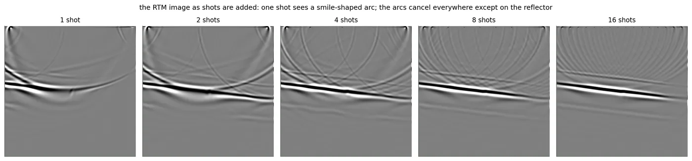
Each sound pulse is a shot. Combining shots from different positions makes the layer clearer:

1 shot2 shots4 shots8 shots16 shots

Click any figure to open it at full size.

1. The idea: listen to echoes

Shout in a canyon and the echo comes back. The longer it takes, the farther away the wall is.

Underground, changes in sound speed and density can reflect part of a wave back to the surface. Those are the echoes we’re after. British Geological Survey

On land, a heavy truck can shake the ground. At sea, a ship can tow air guns that release compressed air under water. Each source event is called a shot.

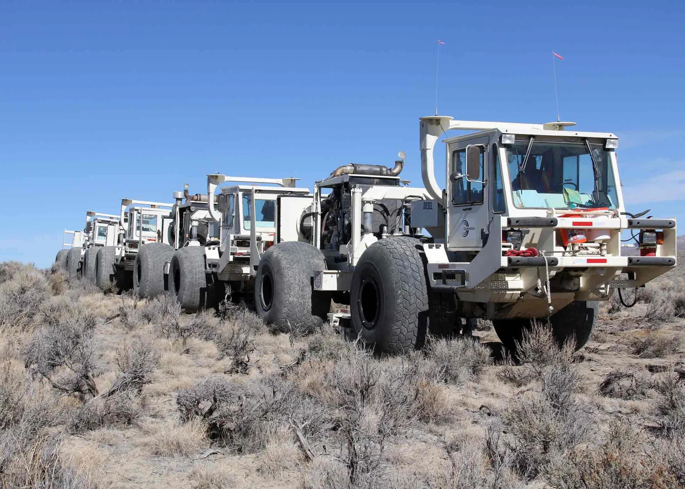
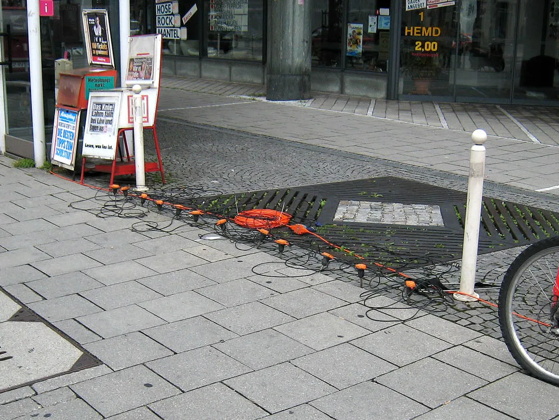
The listeners on land are geophones, which measure ground motion. At sea, hydrophones measure pressure changes in the water. USGS

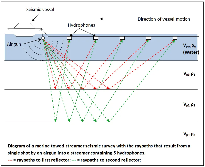
A few terms used below:

• shot: one source event.
• receiver: one listener (a geophone or hydrophone).
• trace: what one receiver recorded after one shot. It’s a wiggly line over time.
• shot gather: all the traces from one shot, placed side by side. This is the raw data.
• velocity model: a map of how fast sound travels at every point underground.
• migration: the step that turns the recordings into a picture of the layers.

These surveys also help monitor CO₂ stored underground. At Sleipner in the North Sea, injection began in 1996. Researchers used repeated surveys to track where the CO₂ spread through the reservoir. Chadwick et al. 2010

The recordings add up. One land survey collected 1.6 petabytes, about 1.6 million gigabytes, across 96,000 recording channels. AOGR 2019

2. What an echo looks like

Picture one bang and a row of listeners on each side of it. Sound goes down, bounces off a layer, and comes back up. For the listener right next to the bang, the trip is short: straight down and straight back. For a listener far away, the sound has to travel a long slanted path, so its echo arrives later.

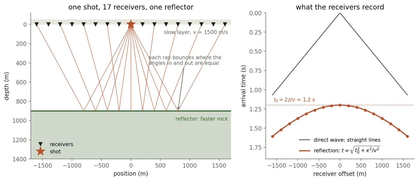
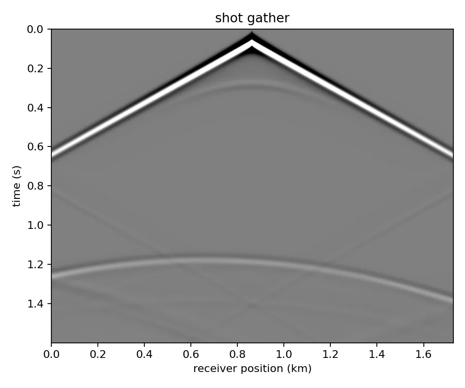
In this flat-layer example, the shortest trip takes 1.2 seconds. To turn that time into a depth, we need to know how fast sound travels. A slower wave from a shallower layer could take just as long. Here is a recording from my simulation:

3. How sound moves

Think of a trampoline. Push one spot down and let go. It springs back, overshoots, and the dip spreads outward as a ring. Every spot on the trampoline is doing one simple thing: it gets pulled toward the average of the spots around it.

For sound, we track pressure instead of the height of a trampoline. Pressure at each point changes in response to the pressure around it. The wave equation describes how:

$$\frac{\partial^2 u}{\partial t^2} = v^2 \,\nabla^2 u + s$$

Here $u$ is pressure. The left side is the second derivative of pressure with respect to time: how its rate of change changes. $\nabla^2 u$ compares pressure at a point with the pressure around it; $v$ is sound speed, and $s$ is the source. This version assumes constant density. Igel, seismo-live

Real rock can also carry shear waves. Including those needs a more expensive elastic model. Both acoustic and elastic models are used in imaging; I kept this example acoustic. Total at GTC 2020, slide 3

4. Turning it into a computer program

A computer can’t store a smooth, continuous ground. So we cut it into a grid: a big table of small squares, each 4 metres wide. Each square holds one number, the pressure there. Time is cut into small steps too, less than a thousandth of a second each.

To move forward one step, every square looks at its neighbours and updates its own number. Here is the idea in its simplest form, for a single row of squares:

# u_now:  pressure in every square right now
# u_prev: pressure one time step ago
# r2:     (speed of sound × time step ÷ square size)², one number per square
for i in 2:n-1
    difference = u_now[i-1] - 2u_now[i] + u_now[i+1]   # second spatial difference
    u_next[i]  = 2u_now[i] - u_prev[i] + r2[i] * difference
end
# rotate the three buffers, then repeat
# u_prev, u_now, u_next = u_now, u_next, u_prev

That’s the update inside the grid. We still need to start the wave and decide what happens at the edges.

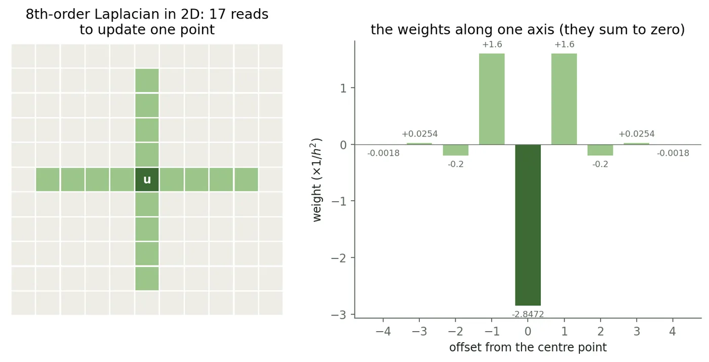
Looking further out. The loop uses one neighbour on each side. Looking farther out can improve accuracy without shrinking the squares. I use four neighbours in each direction, weighted differently: 17 points including the centre in 2D, or 25 in 3D. This is called an eighth-order stencil. Micikevicius 2009

Two rules you can’t break. You can’t pick the square size and the time step freely.

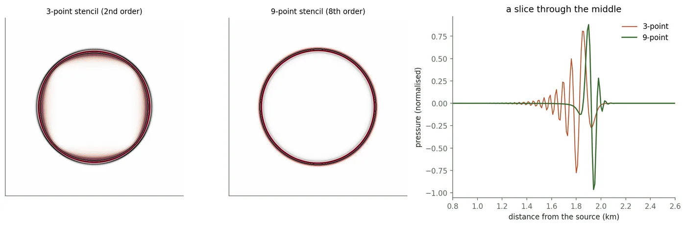
1. The squares must be small enough. If too few fit inside a wavelength, the simulated wave travels at the wrong speed. How many you need depends on the stencil and how much error you can accept. Igel, seismo-live
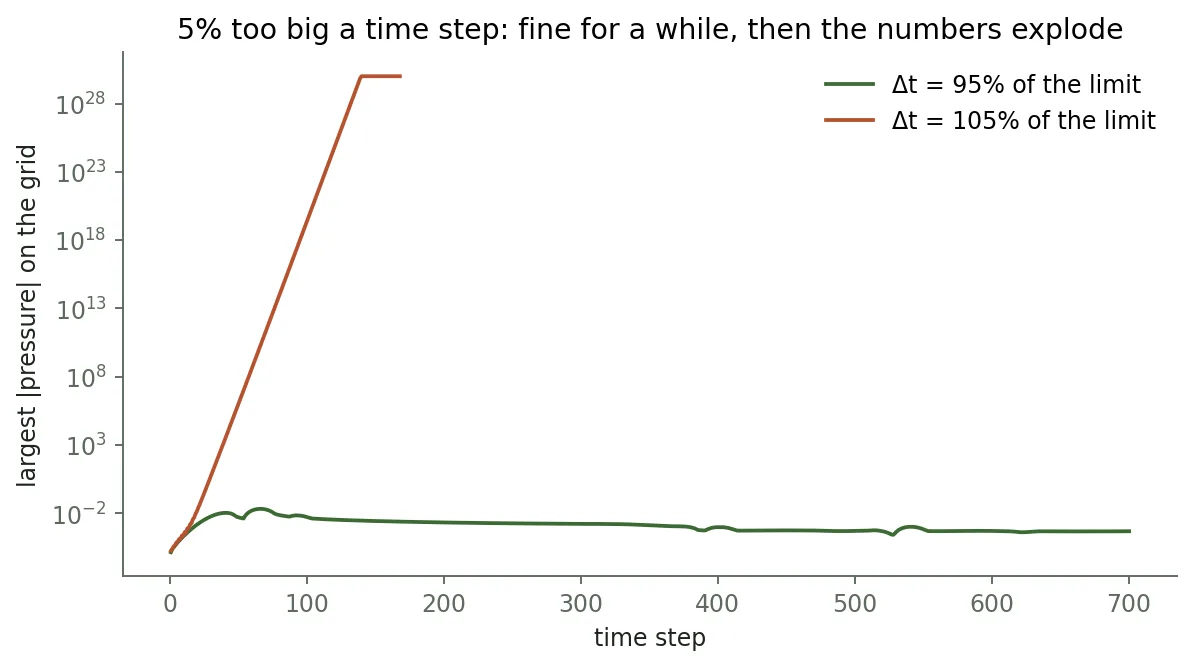
2. The time step must be short enough. Too large a step lets numerical errors grow until the simulation blows up. The limit depends on sound speed, grid spacing, dimension, and stencil. This is the CFL condition. Devito, critical_dt

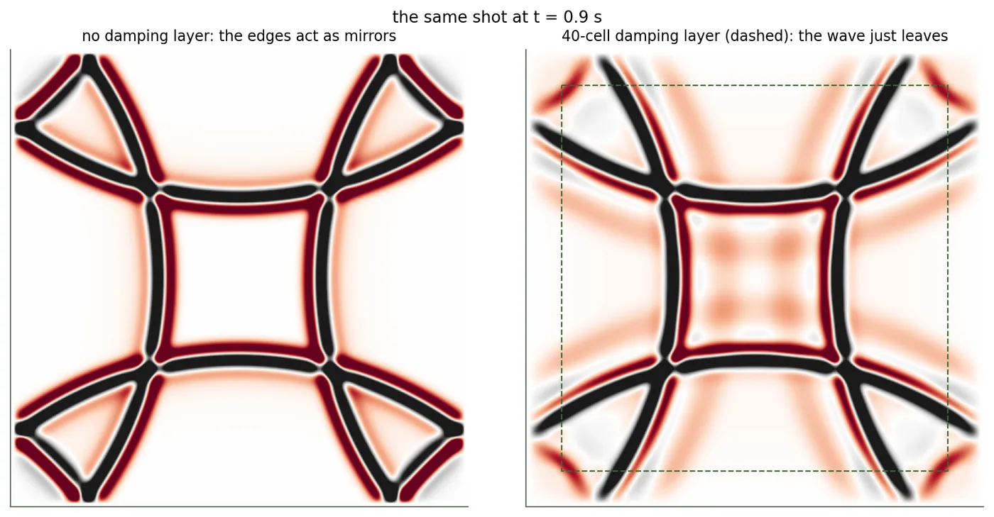
Here is what happens when you break each rule on purpose:

Second-order stencilEighth-order stencilPressure along a slice

The edges. Our grid has edges, but the real ground doesn’t. A wave that hits the edge of the grid bounces back as if from a mirror and ruins the picture. The fix is a soft border, 40 squares wide, where the wave is slowly damped until it fades away, like a room with foam on the walls. Cerjan et al. 1985

Reflecting edgesDamping border

5. Running it on a graphics card

A GPU runs many copies of a small program called a kernel. Each copy is a thread. Here, one thread updates one grid point. It reads the old pressure values and writes to a separate array, keeping the values its neighbours still need. CUDA.jl kernels

This is the update kernel in Julia with CUDA.jl. It adds the wider stencil, the soft border, and the source. The code that allocates arrays and launches it is left out here:

function step!(u_next, u, u_prev, r2, damp_x, damp_z, c, nx, nz, src_x, src_z, bang)
    # grid point assigned to this thread
    ix = (blockIdx().x - 1) * blockDim().x + threadIdx().x
    iz = (blockIdx().y - 1) * blockDim().y + threadIdx().y
    if 4 < ix <= nx - 4 && 4 < iz <= nz - 4
        # eighth-order Laplacian, before scaling by grid spacing
        diff = 2c[1] * u[ix, iz]
        diff += c[2] * (u[ix-1, iz] + u[ix+1, iz] + u[ix, iz-1] + u[ix, iz+1])
        diff += c[3] * (u[ix-2, iz] + u[ix+2, iz] + u[ix, iz-2] + u[ix, iz+2])
        diff += c[4] * (u[ix-3, iz] + u[ix+3, iz] + u[ix, iz-3] + u[ix, iz+3])
        diff += c[5] * (u[ix-4, iz] + u[ix+4, iz] + u[ix, iz-4] + u[ix, iz+4])
        γ = max(damp_x[ix], damp_z[iz])                     # soft border: zero in the middle
        s = (ix == src_x && iz == src_z) ? bang : zero(bang) # the bang, at one square
        u_next[ix, iz] = (2 - γ) * u[ix, iz] - (1 - γ) * u_prev[ix, iz] + r2[ix, iz] * diff + s
    end
    return
end

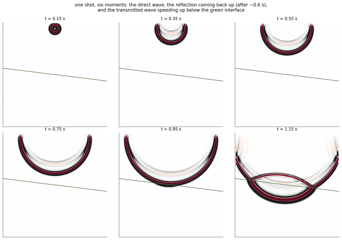
The test ground: 3 km wide and 3 km deep, with slow rock (1,500 m/s) on top and faster rock (2,500 m/s) below. The boundary between them tilts a little. The bang is near the surface in the middle.

0.15 s0.35 s0.55 s0.75 s0.95 s1.15 s

6. Making it fast

I ran this on the RTX 5070 in my desktop.

The GPU can spend more time waiting for values from memory than doing arithmetic with them.

The roofline model asks which runs out first: arithmetic or memory bandwidth. If each byte fetched lets you do very little maths, memory can hold the program back while most of the arithmetic capacity goes unused. Williams, Waterman & Patterson 2009

I use Float32, which stores each number in four bytes. Float64 uses eight bytes and keeps more digits of precision.

For each update, count three reads: current pressure, previous pressure, and the speed coefficient. Add one write for the new pressure. Four numbers at four bytes each gives 16 bytes per update. That’s an estimate. It assumes recently used neighbours are still in the GPU’s cache, a small, fast memory, and leaves out the damping arrays. Micikevicius 2009

My memory-copy test reached 536 GB/s, counting reads and writes. Divide that by 16 bytes and you get 33.5 billion updates per second. I used that as a reference. The wave kernel accesses memory differently from a copy, so the comparison is approximate.

Memory brings back groups of nearby values. If neighbouring threads ask for neighbouring numbers, fewer memory transactions can serve them. Scattered reads waste more of each transfer. This is called coalescing. NVIDIA’s finite-difference example

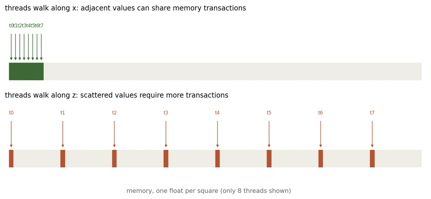
In Julia, the first index changes fastest in memory. For u[ix, iz], walking along x reads adjacent values; walking down z jumps a column at a time. So I mapped neighbouring GPU threads to x. Julia’s performance guide

# strided: neighbouring threads read different columns
iz = (i - 1) % nz + 1;  ix = (i - 1) ÷ nz + 1

# coalesced: neighbouring threads read adjacent values
ix = (blockIdx().x - 1) * blockDim().x + threadIdx().x

I compared five versions on a 4096 × 4096 grid under Windows. Each ran for 20 warm-up steps, then 300 timed steps using CUDA.@elapsed. The rates below count updated points inside the four-cell outer edge.

The timing covers the wave-update loop. Code and run commands are on GitHub. These measurements are from the earlier RTX 5070 run.

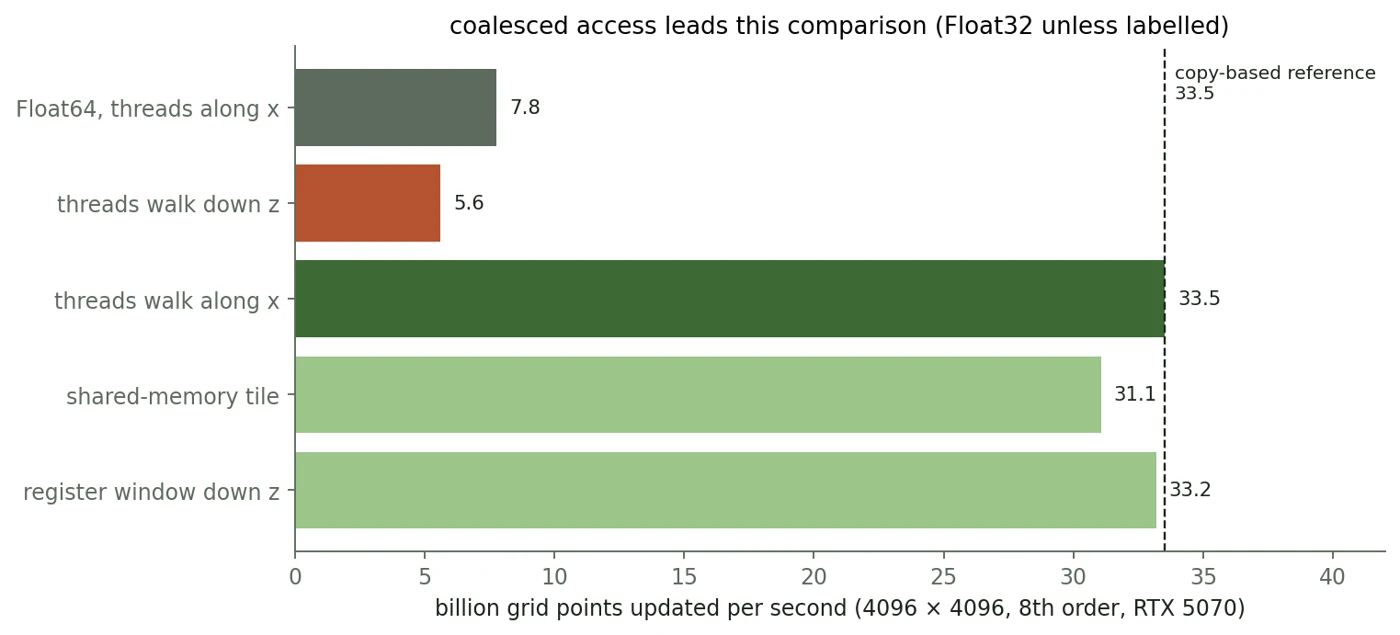
• Strided access: 5.6 billion updates per second. Neighbouring threads walk down z, touching addresses far apart.
• Coalesced access: 33.5. Mapping threads along x is about six times faster in this comparison and close to the bandwidth reference.
• Shared-memory tile: 31.1; register window: 33.2. Both try to reuse values more carefully, using techniques from Micikevicius. Neither helped here. The result can change with the GPU and stencil; Ewart & Araya-Polo found that relying on caches worked better on some hardware than others.
• Float64 with coalesced access: 7.8. About 4.3 times slower than Float32. It moves twice as many bytes per number and uses different arithmetic hardware. This test doesn’t tell us how much each contributes, or how much precision a different simulation would need.

I kept the coalesced version. On 22 September, I tested the current code on a Quadro RTX 8000 under Linux. It reached a median of 35.90 billion updates per second across three coalesced Float32 runs at the same grid size and step count. The hardware, code and operating system differ from the earlier RTX 5070 run, so a direct comparison will need a fresh run on that PC. Raw results and environment

7. From echoes to a picture

We have the recordings. Now we want the layer. We still need a rough map of sound speed to put it at the right depth. Devito’s RTM tutorial

For this test, I blur the known speed map. I also simulate recordings with that blurred map and subtract them from the original recordings to reduce the direct wave. Getting a useful speed map from real data is a separate problem.

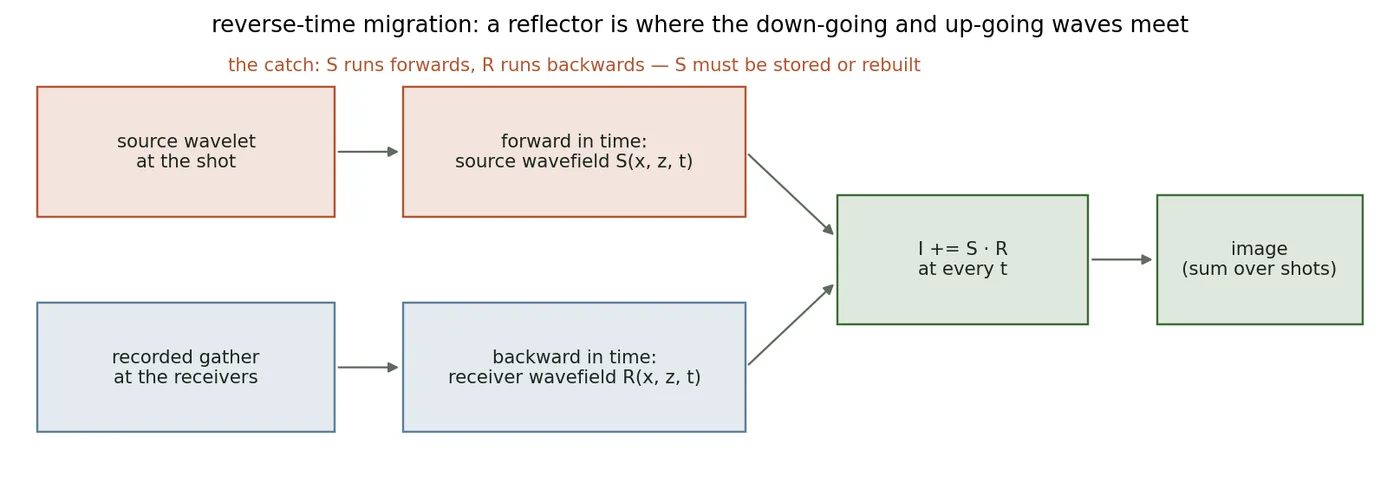
The method is called reverse-time migration, or RTM. It uses an imaging principle proposed by Jon Claerbout in 1971: a layer is wherever the sound going down and the echo coming up are in the same place at the same time. Claerbout 1971

So, for each bang:

1. Forward. Simulate the bang, going forward in time. This is the sound going down.
2. Backward. Play the reflections back at the receiver positions, starting with the last recording. The simulated waves travel back toward the layer.
3. Multiply and add. At each point and time, multiply the two waves and add the result to the image. Their overlap builds up near the layer. Some unwanted overlap shows up as artifacts too.

In pseudocode, that’s one loop:

image = zeros(nx, nz)
for t in last_step:-1:1
    down = source_wave_at(t)            # step 1, the bang going down
    up   = recorded_echoes_backward(t)  # step 2, propagate recordings backward in time
    image .+= down .* up                # step 3, where they meet, a layer
end

Here it is caught halfway through:

Source waveRecorded echoes backwardAccumulated image

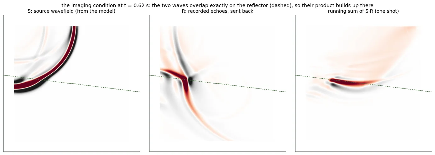
Adding shots from other positions fills in more of the layer, as the opening figure shows. I applied a Laplacian filter to bring out sharp changes and adjusted the contrast separately in each panel. Compare the shapes, rather than their brightness.

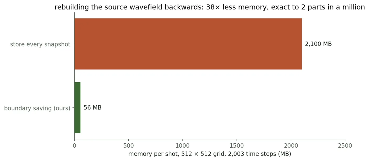
Step 3 needs the sound going down and the echo coming up at the same moment. But one is computed forward and the other backward. The easy fix is to save every moment of the downward sound. For my small test that’s 2.1 GB per bang. For a real 3D survey it can be hundreds of terabytes. Anderson et al. 2012

Inside the grid, we can run the update backward. The damping border is the problem: it removes information. So I keep the final time levels and save a four-cell strip around the interior at every step. Those strips supply the missing values while I rebuild the wave backward. Boundary-saving methods

At 512 × 512, the strips take about 56 MB instead of 2.1 GB for the full snapshot history, roughly 38 times less. I compared the rebuilt wave with a saved copy at a point in the backward run. The largest difference inside the border was about $2\times10^{-6}$ of the largest pressure in the saved copy.

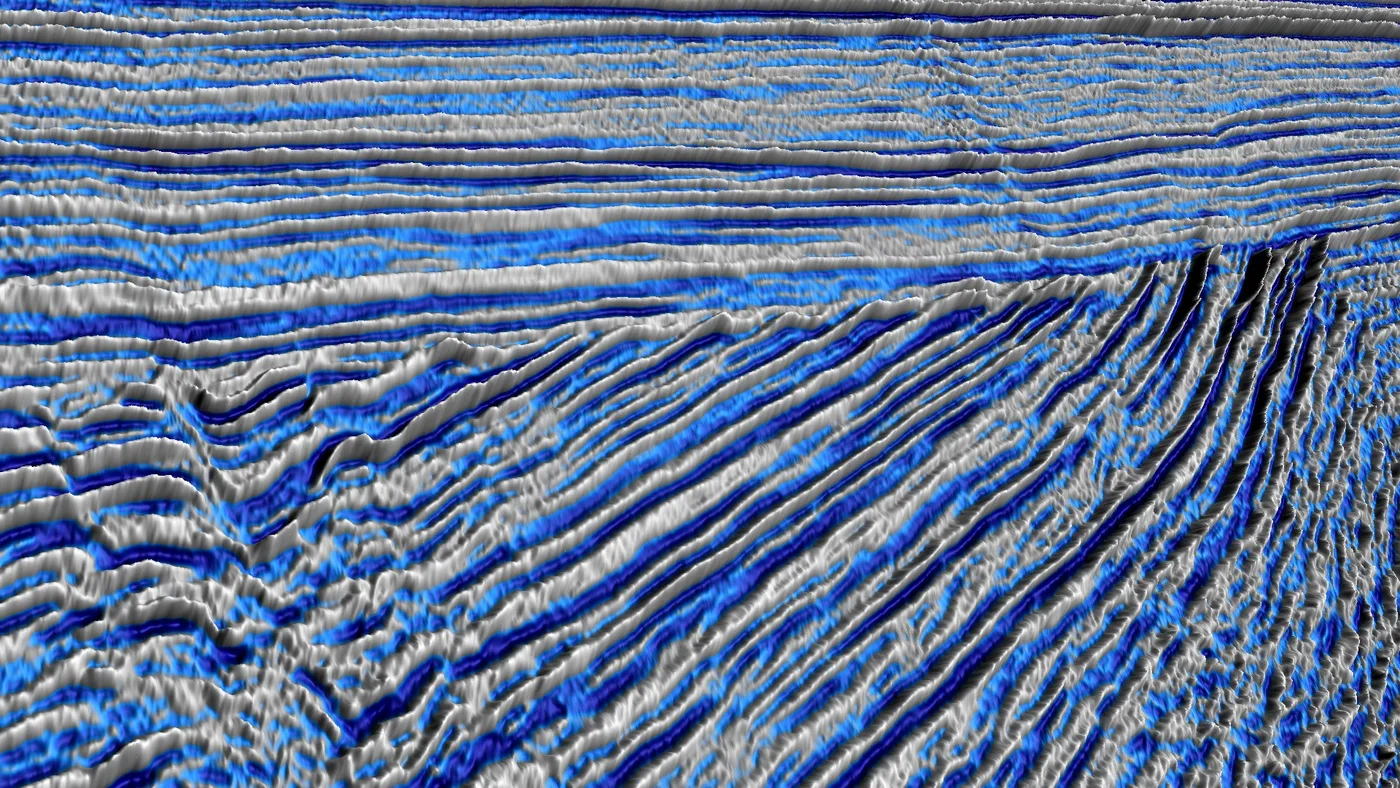
In this real seismic image, older tilted layers were eroded before younger, flat layers formed above them:

8. Where this goes next

Where does the speed map come from? One approach is full-waveform inversion (FWI): start with a velocity estimate, simulate recordings, compare them with the observations, and use the residuals to calculate an update. If you know machine learning, think gradient descent with a wave simulator as the model. A poor starting estimate can lead to the wrong solution. Virieux & Operto 2009

Repeating those simulations is expensive. Total described running FWI and imaging on Pangea III, with 3,348 GPUs. GTC 2020, slides 8–11

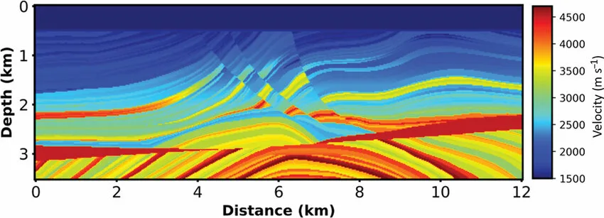
More complicated synthetic models test how well these methods handle folds and faults. Marmousi, built in France in 1988, is a widely used example. Madagascar

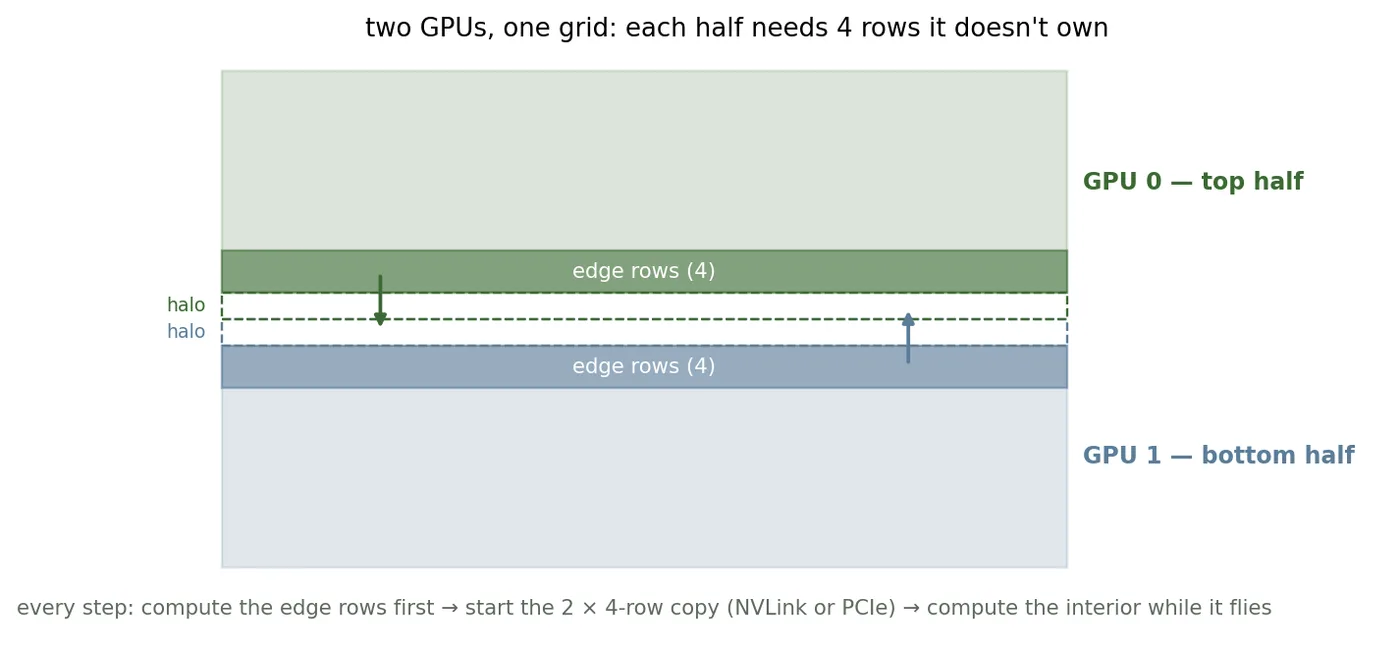
Two graphics cards. Split the grid in half and each GPU has less work. The catch is the cut: each half needs four rows from the other at every step. This swap is a halo exchange. Both GPUs can work on their interiors while the rows travel, though how much time that saves depends on the grid and the connection between cards. Micikevicius 2009

The split now passes a 128 × 128 correctness test on two physical Quadro RTX 8000s, with and without transfer overlap. Both match the single-device result in that test. One card had other jobs running, so I still need clean two-GPU timings. Test output

In 3D, the same eighth-order stencil uses 25 grid points per update. Total’s example workloads reach a billion grid points and more than 10,000 shots. GTC 2020, slides 10–12 Tools such as Devito generate optimised code from equations; ParallelStencil.jl helps write stencil kernels for CPUs and GPUs in Julia.

Where to learn more

1. Louboutin et al., Full-waveform inversion, parts 1–3 (2017–18), with runnable notebooks. The best path from zero to RTM that I found. Part 1
2. Heiner Igel, Computational Seismology: A Practical Introduction (Oxford, 2016), and his free online course Computers, Waves, Simulations.
3. Daniel Köhn’s free notebooks on seismic waves: grids, stability, soft borders and a Marmousi exercise. GitHub
4. Ian Jones’s short tutorials on imaging and inversion.
5. Öz Yilmaz, Seismic Data Analysis, the industry’s textbook, free on the SEG Wiki.
6. Gazdag & Sguazzero, Migration of seismic data (1984), written for readers with no seismic background. PDF
7. Micikevicius, 3D finite difference computation on GPUs using CUDA (2009): shared-memory tiles, register reuse, and overlapping communication. PDF
8. Williams, Waterman & Patterson, Roofline (2009): the chart to draw before speeding anything up. PDF